



One of the requirements for accurate GNSS observation is a clear sky to achieve good tracking of the signals sent by satellites. This requirement seems to be an inescapable condition for GNSS; however, Trimble has introduced significant improvements to the RTK processing engine for its new GNSS receivers.
Specifically, ProPoint™ enables RTK positioning based on three basic concepts:
⨭ Accuracy: difference between the true and measured value. Trimble ProPoint™ ensures that this value will be minimized.
⨭ Reliability: certainty of the real-time variance-covariance estimation. This is the most important criterion since the true value is not always known.
⨭ Productivity: simply involves acquiring more fixed points per unit of time because the receiver optimizes coordinate determination. In practical terms, this means more time where the solution converges to survey-grade accuracy, with a corresponding gain in productivity.
Strictly speaking, these three concepts must occur together, making fieldwork as efficient as possible. From a technical standpoint, ProPoint™ is nothing more and nothing less than an algorithm available in Trimble receivers that, through intensive processing of all observed GNSS signals, achieves survey-grade coordinate determination even in locations with difficult satellite observation.
Perhaps the most difficult criterion to evaluate is reliability, given that it is a probabilistic estimation. For example, in conventional GNSS systems that use the fixed/float technique, high reliability does not always mean high accuracy. This means that some accuracy determinations are extremely optimistic and, in reality, show a significant difference between the true value and the observed value. The ProPoint processing engine clearly demonstrates having overcome this.
To test ProPoint™, a measurement experiment was conducted using a Trimble DA2 mobile device receiving differential corrections from a Trimble R12i GNSS base. The chosen scenario was a stream with extensive vegetation cover that makes satellite observation difficult. The Trimble R12i base was installed at a point with known coordinates to send differential corrections via the internet in CMRx format, which is capable of handling all available GNSS constellations and signals.
Site Conditions
First of all, a location with complications for satellite observation was chosen, one that would be challenging for the receiver in terms of real-time coordinate determination. For this reason, a stream was selected that had not been cleared, resulting in dense vegetation cover along with large trees on the sides that could cause problems for satellite observation, as shown in Figure 1.

Figure 1. Stream conditions.
Achieved Productivity
A topographic representation of over 3 km was achieved through transverse profiles every 25 m, determined using a Trimble DA2 receiving differential corrections from a Trimble R12i base. This representation was carried out over two days from different setups for the Trimble R12i base that transmitted differential corrections via the internet (see R12i as an internet base station news):

Figure 2. Topographic survey of the stream.
Thus, the following results were obtained:
|
Day |
Mar 21, 2022 |
Mar 22, 2022 |
|
Total Time |
5 hours 10 minutes |
3 hours 45 minutes |
|
Points Surveyed |
453 |
408 |
|
Time per Point |
40 seconds |
33 seconds |
Table 1. Productivity achieved by Trimble DA2
Another way to represent productivity is by plotting graphs that show the distribution of points over time. From these graphs, it can be seen that there are practically no "idle times":
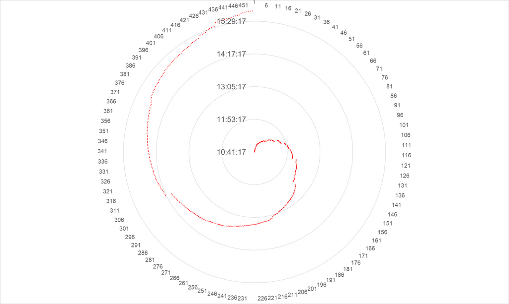
Figure 3. Distribution of points over time for March 21, 2022

Figure 4. Distribution of points over time for March 22, 2022
Reliability
It has already been indicated that reliability will be evaluated in terms of the determination of variance-covariance from the coordinate calculation. Simplifying the analysis, only horizontal accuracy, vertical accuracy, and the number of observed satellites will be shown. In the case of accuracies, these will be indicated with a 68% confidence interval (1-sigma).
For this, Figures 5 and 6 show, through their distribution over time, the horizontal accuracy in blue and the vertical accuracy in red, associated with the left axis indicating values in meters. Finally, in green, the number of satellites related to the coordinate determination is shown, whose values are indicated on the right axis:

Figure 5. Distribution of accuracies and satellites over time for March 21, 2022

Figure 6. Distribution of accuracies and satellites over time for March 22, 2022
The above can be summarized in the following statistics:
|
Day |
Mar 21, 2022 |
Mar 22, 2022 |
|
Mean Horizontal Accuracy |
0.021 ± 0.048 |
0.017 ± 0.039 |
|
Mean Vertical Accuracy |
0.037 ± 0.071 |
0.030 ± 0.059 |
|
Mean Number of Satellites |
16 ± 3 |
17 ± 3 |
Table 2. Summary of accuracy and number of satellites
In terms of grouping solutions by their horizontal accuracy, the following can be established:
|
Day |
Mar 21, 2022 |
Mar 22, 2022 |
|
Less than 5 cm |
92.3% |
93.9% |
|
Between 5 to 10 cm |
5.3% |
3.7% |
|
More than 10 cm |
2.4% |
2.5% |
Table 3. Distribution of horizontal accuracy
Accuracy
This is the most difficult element to evaluate, as the true value must be known to compare it with the determined value and obtain what is known as error. Strictly speaking, accuracy is defined as the degree of dispersion of a sample; however, it has been agreed that defining it this way is impractical.
To address this point, the relationship of a low-accuracy point with its neighborhood will be evaluated. It should be recalled, from Table 3, that less than 2.5% of the determined points have a horizontal accuracy of less than 10 cm (19 points out of a total of 856).
The survey was conducted using transverse profiles every 25 m. Each point comprising the profiles describes a geometry relative to its surroundings. In Profile 1 (Figure 7), there are 7 points, only one of which was determined with lower reliability (0.396 m horizontal accuracy and 0.720 m vertical accuracy). However, the expected shape remains unaltered considering the application for which the topographic representation is intended.

Figure 7. Profile 1
In summary, no points were eliminated, as all of them contributed to forming a surface that faithfully represents the stream. The same can be confirmed for Figure 8.

Figure 8. Profile 2
Compartir:
OPINION COLUMN | RIEGL LiDAR: Geocom at the Forefront of Mining Projects
Applying RTX with Trimble DA2