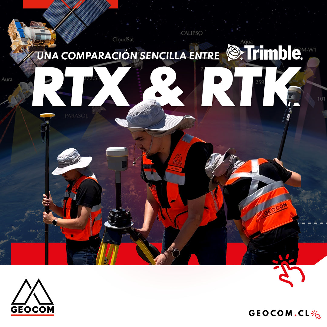
A simple comparison between Trimble RTX & RTK

GNSS & Geocom Optics

 

GNSS is widely known as a geodetic observation instrument, mainly for its differential or relative methodologies, which indicates that at least a pair of receivers operating simultaneously is required to obtain results compatible with surveying activity. However, GNSS also presents an absolute methodology: it is possible to use only one receiver to obtain highly precise geodetic positions. The latter is known as PPP.

Trimble, for its part, has deepened the PPP technique through Trimble RTX, which can be used either in real-time or in post-processing. Now, in terms of compatibility, the questions that arise are: Is RTX compatible with determinations made in RTK? Can RTX and RTK data coexist in the same project?

The answer to these questions is associated with knowing how a point changes its coordinates over time due to geodynamic effects: the concept of epoch appears. Fortunately, Trimble RTX along with Trimble Geodetic Library solve this problem.

 

GNSS and differential methodologies

In the geodetic and topographic field, GNSS has always worked under the differential concept. This directly involves the determination of baselines, associated with the geocentric system, which allow determining the coordinates of a second point by knowing the position of the base.

In this sense, coordinate determination is linked to the position of the base, relying on the relative concept. Strictly speaking, this type of determination is very much tied to the conventional topographic perspective, which has given confidence to geospatial professionals.

 

Figure 1. Differential methodology for GNSS

 

Trimble RTX

Trimble RTX is a satellite positioning technique that does not require a base, allowing for the determination of precise coordinates. Whether in post-processing or real-time, Trimble RTX processes a satellite observation, using code and phase, to determine precise coordinates associated with the instantaneous epoch (the moment at which the observation was made).

 

Figure 2. Trimble RTX: a geostationary satellite sends the correction to a mobile receiver

 

Leaving aside the technicalities of the technique (incorporation of precise orbits, atmospheric modeling, and clock correction), the main difference between Trimble RTX and differential techniques is the emergence of the concept of epoch. While the differential methodology fully depends on the base's position, Trimble RTX performs a calculation intimately associated with the epoch, obtaining solutions completely independent of the geodynamic activity affecting the location.

 

What is the reference epoch?

To explain the concept of reference epoch, it is important to refer to a time series. For this, the SANT station, which is processed by different SIRGAS processing centers, will be used, resulting in the following time series:

 

Figure 3. SANT time series calculated by SIRGAS

 

As can be seen in the graph, the horizontal component (blue for north and green for east) shows a linear behavior with respect to time, except for some discontinuities caused by non-linear geodynamic effects. Let's assume that the reference epoch is 2016 and that determinations are made in 2019: the difference between both positions exceeds 5 cm. Therefore, the position determined in 2019 can be "regressed" to 2016 by knowing the velocity of that station.

 

Figure 4. Linear velocity in the 2016-2019 period

 

When dealing with linear velocities, the problem has a simpler solution. However, there are times when velocities cannot be expressed linearly, such as during an earthquake.

Finally, an absolute determination at an instantaneous epoch will be different from that of a given reference epoch. This is the case with SIRGAS-Chile 2021, whose reference epoch is precisely the year 2021. Any observation made with Trimble RTX at a given instantaneous epoch that needs to be represented at a reference epoch must necessarily be transformed. For this, it is necessary to establish the use of velocity models that correspond to grids that allow transforming horizontal coordinates between epochs.

 

Figure 5. Non-linear velocity for an extremely short period

 

TGL: Trimble Geodetic Library

Given the need to know geodynamic velocities, grids are created that allow interpolating coordinates between given epochs. The VEMOS model created by SIRGAS is well known, which allows interpolating horizontal velocities for the change of epoch of a position.

 

Figure 6. VEMOS and its different versions

 

It is precisely this model that is implemented by Trimble in its geodetic library (TGL), which is transversal to both Trimble Business Center and Trimble Access.

 

Figure 7. Trimble Access and its relationship with VEMOS2017

  

Trimble RTX, after determining a position at the instantaneous epoch, uses the models available in TGK to perform the calculation directly in SIRGAS-Chile 2021 by applying a correction fully compatible with other relative determinations made with GNSS.

 

Application Example

A comparison was made of coordinate determination in SIRGAS-Chile 2021 using the differential methodology, mixing post-processing and real-time techniques with the use of Trimble RTX in real-time. The proposed scenario involves the installation of control points for a photogrammetric flight.

 

Figure 8. Trimble R12i in operation

 

Regarding relative operation, the conventional methodology is as follows:

Densification of SIRGAS-Chile 2021 through the observation of a baseline

Point A1 is observed while the drone flight is being carried out, to be linked to SIRGAS-Chile 2021 from the continuous reference station SNTI, which is part of the GEOCOM GNSS Network.

 

 

Figure 9. GNSS Baseline between SNTI and A1

 

This observation lasted 2 hours and 17 minutes, observing GPS+GLO+GAL+BDS with multifrequency, achieving a precision of 6 mm horizontally and 26 mm vertically at a 95% confidence interval. This directly provides the position of A1 in SIRGAS-Chile 2021.

RTK observation of control points

From the installation of the Trimble R12i base over A1, differential corrections are emitted for a mobile, also a Trimble R12i, which determines the SIRGAS-Chile 2021 coordinates in RTK. In the office, when the coordinates of A1 are determined, this survey is recalculated.

 

Figure 10. RTK observation of control points

 

On average for the five observed control points, an average of 12.3 mm horizontally and 14.4 mm vertically was obtained at a 95% confidence interval with observations using the TOPO point methodology.

Additionally, RTX observations are performed with Trimble DA2 along with Trimble Access. Only convergence is needed, which is achieved in a couple of minutes after initializing the receiver and it begins to receive corrections from a geostationary satellite (or via the internet).

 

Figure 11. Trimble DA2 observing control points with Trimble RTX

 

RTX observation of control points

A Trimble DA2 GNSS receiver is used in conjunction with Trimble Access, configuring a project using SIRGAS-Chile 2021 (important for obtaining coordinates in the appropriate reference frame). Each control point is observed for at least 5 seconds using Trimble Access's TOPO point methodology. Finally, SIRGAS-Chile 2021 coordinates are obtained for each point with minimal effort.

Finally, for comparison, the coordinates between RTK and RTX are compared:

 

Table 1. Differences between RTK and Trimble RTX

Conclusions

The use of RTX as a GNSS positioning technique perfectly describes the time component present in modern definitions of Geodesy. Trimble RTX, through determinations at the current epoch, provides centimeter-level precision and real-time GNSS positions which are automatically linked to the national geodetic framework SIRGAS-Chile 2021 through the adoption of the VEMOS 2017 displacement model.

The epoch reduction carried out by RTX allows the user to align with the official geodetic definition in force in Chile without the need for transformations or adjustments after the field observation process. This can be easily applied, as presented in the article's experience, in the acquisition of control points for photogrammetry. Regarding the comparison made, these show centimeter-level differences between both methodologies, inherent to each determination.